PCA (à la french school)

March 20, 2015 by Herimanitra

Today, we will see how to perform Principal Component Analysis using FactoMineRpackage.

PCA, what is It?

PCA (Principal Component Analysis) is a dimensionality reduction technique aiming to summarize multidimensional information from a dataset consisting of N rows and M columns. It helps also select relevant variables that summarize the dataset. The idea consists of projecting dataset into 2-dimensional subspace that reproduces as most as possible information from the raw dataset.

Columns have to be numeric in PCA or transformed into numeric ( using one hot encoding for instance). Qualitative variables can help during the description of principal component axis. Thus, they always put into supplementary or complementary but a numeric variable can also be put into supplementary to help during interpretation.

All variables involved in PCA must be normalized ( substract the mean and divide by standard deviation).

What are we looking for when using PCA?

The goal is twofold:

First, we are trying to find out profiles of individuals that are similar in the dataset. We are particularly interested in what makes these individuals different from others and why they are homogeneous. Similarity between individuals are assessed with usual distance metrics such as Euclidian distance.

In addition,we are also interest in finding variables that are linearly "linked" and/or correlated to each other using the coefficient of correlation.

In PCA, we always have dual graphics:

• Individual or observation graphic which plots position(coordinates) of each observation of the dataset in a principal component (1st, 2nd, 3rd, etc.).
• Correlation circle which represents the correlation between variables and their respective contribution to the construction of principal components.

Do you know Factoshiny package?

It's a new package which performs factorial analysis thanks to FactoMineR and Shiny.

To illustrate, let's use iris dataset from R:

Individuals factor map:

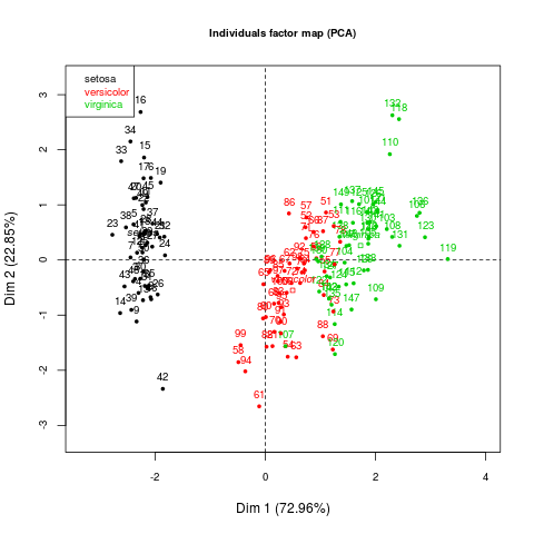
First 02 axis explain more than 90% of the variance and the 03 species (setosa,versicolor and virginica) are clearly separated. Furthermore, first axis opposes setosa from the others.

Variables factor map:

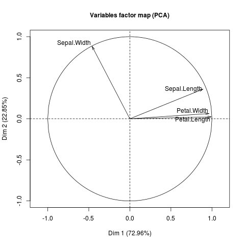
Sepal and petal lengths but also petal width contribute most to the construction of the first axis (they are closely correlated from each other). It may be true that setosa species differ from the other species due to these variables.

If you want to explore iris dataset using PCA with Factoshiny, here is the code:

data(iris)
#install.packages("Factoshiny")
require(Factoshiny)
output=PCAshiny(iris)